Image colorization: learning what grayscale leaves out
How local detail and scene context help a neural network predict colour, and why plausible is not the same as correct.
A grayscale photograph still tells us a lot. We can see a person, a tree, a patch of sky. But a shirt that looks dark might have been blue, green or red. Removing colour throws away information. Putting colour back means making a prediction, not undoing a reversible operation.
In 2019, I built an image colorization model for the DD2424 course at KTH. I used TensorFlow and Keras to reproduce the approach in Deep Koalarization, with some modifications. The model combined a convolutional encoder with a pretrained Inception-ResNet-v2 network, then decoded their combined features into colour.
The interesting part is how those two paths help each other. One looks at local detail. The other provides context for the whole image. Neither can tell us the original colour of every object.
1. Keep the lightness, predict the colour
Start with a pixel in the sky. Rather than ask the model to predict its red, green and blue values from scratch, I separate lightness from colour using the CIE L*a*b* colour space.
L* represents lightness. a* runs roughly from green to red, and b* from blue to yellow. My input is L*. The target is the pair (a*, b*). At the end, I combine the predicted pair with the original L*, then convert back to RGB for display.
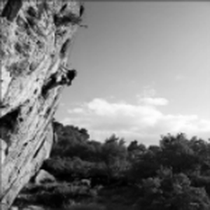
L* alone is a complete grayscale photo. This is the model's input.
The other two channels are what the model has to invent. Shown on their own at constant lightness, they look like this:
 a*: green to red
 b*: blue to yellow
The notebook also scales the values before training: L*/50 - 1 for the input, and a*/128 and b*/128 for the targets. Those are numerical conventions, not new colours. Reconstruction reverses the scaling before converting to RGB.
This split gives the model a narrower job. The sky’s shape and lightness are already there; the model has to estimate its missing colour. But to do that, it first needs clues about what the pixel belongs to.
2. Detail is useful, but context changes its meaning
A convolution is a small filter moved across an image. It can respond to patterns such as edges and textures. Stacking these layers lets the encoder build a more useful representation than individual pixel values.
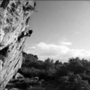 Input L*
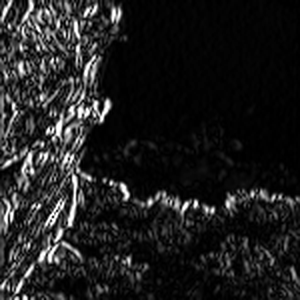 vertical edges
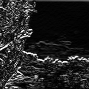 horizontal edges
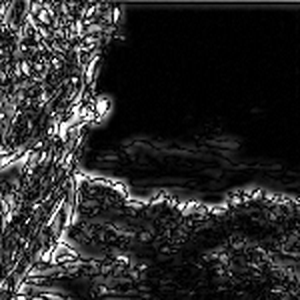 local contrast
A smooth light patch, though, could be sky, a wall or fabric. Its nearby pixels help, but so does knowing whether the entire image looks like an outdoor landscape or an indoor room. That is why my model has a second path.
I send a grayscale version of the image to Inception-ResNet-v2, pretrained on ImageNet. Its expected input is 299 × 299 × 3, so I resize and repeat grayscale across three channels. Repeating grayscale does not restore colour. It only makes the input compatible with the pretrained network.
The project report calls the pretrained representation high-level features. There is a useful implementation detail here: the v2 notebook creates Inception-ResNet-v2 with include_top=True and uses inception.predict. That gives the 1,000 class outputs. The report describes a vector before softmax, so its wording and this notebook are not identical. The safe description is a 1,000-value pretrained representation, rather than claiming every version uses pre-softmax activations.
3. Put the scene context at every location
Now there are two things of different shapes. The encoder produces a grid of local features. The pretrained network produces one vector for the image. Fusion repeats that vector at every position in the grid and concatenates it with the local features.
In the v2 notebook the input is 256 × 256. Three stride-2 convolutions reduce height and width by a factor of eight, so the encoder output is 32 × 32 × 256. Repeating the 1,000-value context vector over that grid produces 32 × 32 × 1,000. Concatenating them gives 32 × 32 × 1,256. (The report used a 128 × 128 input, which gives a 16 × 16 grid with the same channel counts.)
A 1 × 1 convolution does not look across neighbouring positions. It learns how to combine channels at the current position. After that, the decoder uses convolutions and upsampling to produce two colour values at each output pixel.
For my sky pixel, the path is now complete: local features describe its region, scene features provide context, and the decoder predicts (a*, b*). Training tells the model how close that guess came to the original.
Here is the whole path, using the layer sizes from the v2 notebook. Step through it. Block height shows height and width of the tensor, block thickness shows the number of channels.
4. Looking at what it predicted
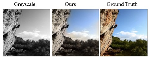
With the architecture in place, the next question is what its predictions look like. The output examples are from the 2,000-image run. First, the three examples side by side. These are the figure from the project, cropped into separate images.
Input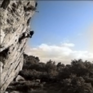 Prediction
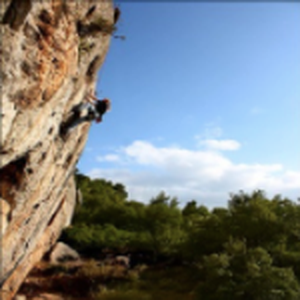 Ground truth
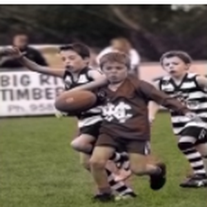
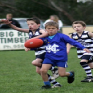
Row 1 lines up exactly, so I can ask where its colour is wrong. Drag the handle to compare the prediction with the original.
The map below measures that difference as distance in the (a*, b*) plane at each pixel: lighter is closer, darker is further from the original. The darkest area is the rock face, where the prediction is grey instead of orange and brown. Sky is the lightest.
PredictionGround truth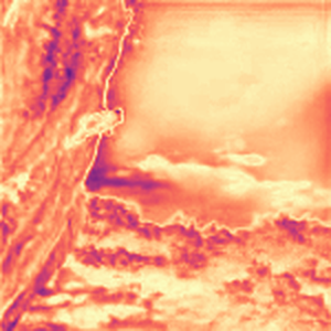 Colour error
The most useful picture is of the colours themselves. Each plot below places every pixel at its (a*, b*) position. Top row: the original colours. Bottom row: what the model predicted.
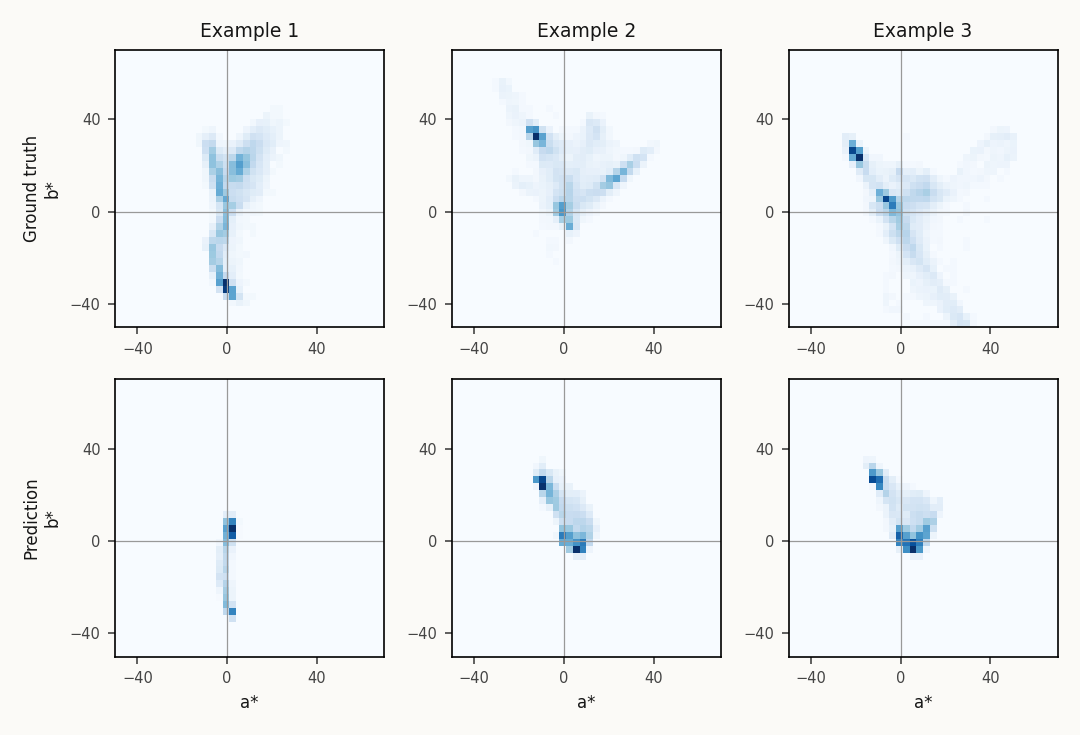
These plots show how muted the predictions are, but they do not establish the cause. Colour ambiguity and an implementation problem are different possible explanations; the output images alone cannot distinguish them.
Plausible colour is not recovered history
The output examples are the most honest ending to this project. The model can put blue into sky and green into grass, while missing a shirt’s actual colour. Local detail and scene context help make a guess; they do not turn that guess into a record of what was there.
I reproduced an approach and got a small model working. I did not establish excellent generalization, a production system, or a measured improvement over a baseline. The useful lesson is to keep those claims separate: fitting one image, producing a plausible example and reliably handling unseen images are different milestones.
Code and references
- My repository: notebooks, architecture and output examples.
- Project report: experiment sizes, training setup, results and the unresolved TFRecords issue.
- The v2 notebook: input normalization, pretrained representation and model implementation.
- Deep Koalarization, Baldassarre, González Morín and Rodés-Guirao (2017): the main architecture I reproduced.
- Let there be Color!, Iizuka, Simo-Serra and Ishikawa (2016): combining local image features with global context.