← All posts

2020-11-14 · 7 min read

My first text classifier for sentiment analysis

Naive Bayes, a linear SVM and a CNN on 1.6 million tweets, and why the data mattered more than the model.

Data & exploration

In spring 2019 I did a course project at KTH with two classmates. It was my first project on text. The question was simple: which classifier is best at telling positive tweets from negative ones? We tried Naive Bayes, a linear SVM and a small convolutional network. I expected the CNN to win, because in 2019 the neural network was supposed to win.

It didn’t. A year and a half later I reread the notebook, and I think the more useful lesson is somewhere other than where we put it at the time.

The data

We used Sentiment140, 1.6 million English tweets from 2009, each labelled positive or negative. The first notebook was exploration: which words show up on each side.

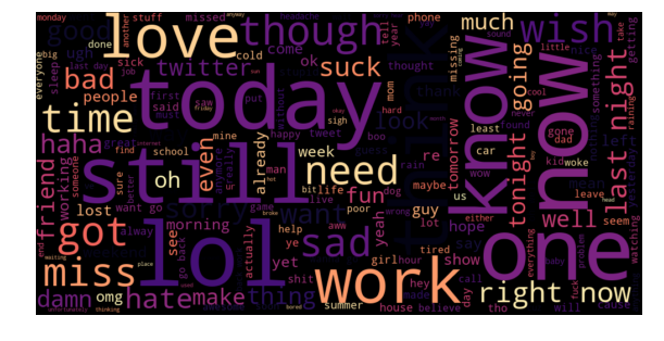
negative tweets

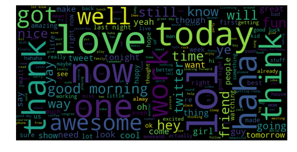
positive tweets

Most frequent words in each class, from our exploration notebook. "Today", "now" and "lol" are large on both sides.

The clouds already hint at the difficulty. The biggest words are the same on both sides. Sentiment sits in the smaller words and in how they combine.

From a tweet to numbers

A model can’t read a tweet; it needs a row of numbers. Everything before the model is about producing that row. Here is the whole pipeline at a glance:

flowchart TB
  T[Raw tweets] --> C[Clean]
  C --> N[N-grams]
  N --> B[Counts or TF-IDF]
  B --> NB[Naive Bayes]
  B --> SVM[Linear SVM]
  C --> E[Word indices]
  E --> CNN[CNN]
  NB --> V[Accuracy on 1M held-out tweets]
  SVM --> V
  CNN --> V

Cleaning. Tweets are messy: mentions, links, HTML entities, inconsistent case, contractions. Our cleaning function handled them in a fixed order:

One made-up tweet through our cleaning function. Orange marks noise that a later step removes; blue marks what a step changed. Expanding "don't" to "do not" was deliberate: it keeps the negation as its own word.

N-grams. Next, each cleaned tweet is split into n-grams: single words (unigrams), pairs (bigrams) and triples (trigrams). Longer n-grams keep a little word order, which matters most for negation.

N-grams are runs of consecutive words. With single words only, "not" and "good" are separate clues that pull in opposite directions; the bigram "not good" is one clear clue.

Bag of words and TF-IDF. Finally, every n-gram in the training set becomes a column, and each tweet becomes a row saying how often each one appears. That’s a bag of words: word order beyond the n-gram is thrown away. Plain counts treat every term alike, so common words dominate. TF-IDF (term frequency × inverse document frequency) scales each count down by how many tweets contain the term:

Each tweet becomes a row of numbers, one column per term (only six of the columns are shown). "good" is in every tweet, so TF-IDF gives it the least weight. Values follow scikit-learn's default formula, with each row normalised over all its unigrams and bigrams.

With about 100,000 training tweets and tens of thousands of columns or more, almost every cell is zero. Models built for this kind of sparse data are fast and hard to beat, which is part of why the linear ones did so well.

The models we picked

We picked three models that use those numbers in different ways, plus a baseline that uses none:

• TextBlob was the baseline. It doesn’t learn anything: it looks words up in a fixed dictionary of positive and negative scores. It showed what we got for free.
• Multinomial Naive Bayes learns how likely each term is in positive and in negative tweets, then multiplies those likelihoods for a new tweet. It assumes terms are independent, which isn’t true, but it trains in seconds and is the standard first model for text.
• A linear SVM learns one weight per term and draws the boundary between the classes with as wide a margin as possible. With tens of thousands of sparse features, of which only a few matter in any one tweet, that’s exactly the setting it’s good at.
• A convolutional network (CNN) skips the counts. Each word becomes a small learned vector, and filters slide over windows of a few words at a time, learning to detect phrases wherever they appear. Ours was small: a 5,000-word vocabulary, 25-dimensional word vectors, and a short stack of convolution layers.

Three ways to reach the same answer. Naive Bayes and the SVM only see which words and phrases occur; the CNN sees word order inside each window. The numbers are made up to show the mechanics, not taken from our models.

Naive Bayes and the SVM only see which terms occur. The CNN sees word order within a window, which is why I expected it to win.

What we measured

After cleaning, we held out a balanced test set of one million tweets and trained on a sample of about 100,000. Before splitting, we removed any training tweet whose text also appeared in the test set. That was a good call, since Twitter is full of identical tweets.

On that test set:

Model	Twitter accuracy
TextBlob, no training (baseline)	0.59
CNN (Keras, 5,000-word vocabulary)	0.777
Multinomial Naive Bayes, TF-IDF 1–3 grams	0.784
Linear SVM, TF-IDF 1–3 grams	0.820

The linear SVM won, and that was the headline of our report. A fair reading is narrower. Anything trained beat the off-the-shelf lexicon by about twenty points, and the three trained models then sat within about four points of each other.

We ran the same three models on Amazon product reviews. All of them scored between 90% and 94%. Changing the dataset moved accuracy by eleven to fifteen points. Changing the model moved it by about four.

Each line is one model on two datasets. The lines are long, while dots of the same colour sit close together: the data moved the result far more than the choice of model did.

Reviews are longer, the words are more specific, and a star rating is a cleaner label than whatever a tweet implies. If I had to predict how well a sentiment model would do, knowing what text it would see would help me much more than knowing its architecture.

The labels were already a model

Sentiment140 was never labelled by people. Its authors collected tweets containing emoticons, treated :) as positive and :( as negative, and then removed the emoticons from the text. So every one of our models learned to predict whether the author had typed a smiley.

That explains the gap with Amazon better than anything we tried. A tweet like “finally finished my exam :(“ carries a negative label that the remaining words hardly support. Beyond a certain point, no classifier can recover information the labelling process never captured. Asking “why can’t we get past 82%?” was really asking about the data.

The stopword that mattered

The experiment I’m happiest with in hindsight is a small one. With Naive Bayes, we compared three ways of handling stopwords:

• keep every word: 0.78
• remove scikit-learn’s standard English stopword list: 0.75
• remove our own list of the twenty most frequent words, excluding not: 0.77

The original notebook plot: Naive Bayes validation accuracy as the vocabulary grows. The standard list (orange) stays lowest at every size.

One example sentence under each setting, with the Naive Bayes validation accuracy on the right.

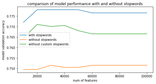
The standard list includes not. Dropping it turns “not good” into “good”. Our cleaning step had already expanded contractions for this reason (“don’t” became “do not”), and then the stopword list removed the part we had been careful to keep. The custom list skipped not deliberately, and in the notebook that exclusion is a single line: del custom_stop_words[2].

It’s the least impressive-looking line in the project, and it is also the best example of the actual job: find out what a preprocessing step removes before assuming it removes noise.

What I would question a year on

Rereading your own work from eighteen months ago is humbling. A few things I would change.

The CNN comparison was unfair. It had a 5,000-word vocabulary, 25-dimensional embeddings, tweets cut at 50 tokens, and 100,000 training examples. The SVM had 1–3 grams over the full vocabulary. The training curve shows the same thing from another angle:

CNN loss over 20 epochs, from the notebook. Training loss (blue) falls; validation loss (orange) rises from the first epoch.

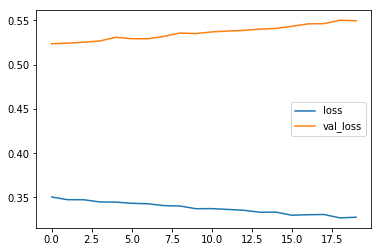
Validation loss went up from the very first epoch, so the network was memorising the training set rather than learning anything that transferred. With that curve, the right move was to stop, get more data or regularise more, not report its accuracy next to the others. So “the SVM beat the CNN” really means “a well-fed linear model beat a network that was overfitting”. That can still be the right practical choice, but it’s a different claim.

One normalisation experiment never ran. The lemmatisation and stemming cells build a normalised copy of the data and then split the original data for training. Their results match the unnormalised run exactly, and we concluded that normalisation made no difference. We never tested it.

The validation AUC was computed from hard labels. During the feature search, the ROC curve was built from predicted classes instead of scores, so the “AUC” matched accuracy almost exactly and added nothing. The final test runs used probabilities correctly. Even so, our README pairs the linear SVM’s accuracy (82%) with an AUC of 0.86, which belongs to the RBF kernel. The linear model’s own AUC is 0.88 in the saved notebook and 0.90 in our slides; those come from different runs, and we never wrote down which one the reported accuracy came from.

The RBF SVM was scored on a 5% sample of the test set, because the full set was too slow. It appears in our comparison table next to models scored on the full million.

None of these change the main conclusion. They do show that the numbers we were proudest of were the least carefully checked.

The notebooks, figures and report are on GitHub.

References

1. Alec Go, Richa Bhayani and Lei Huang. Twitter Sentiment Classification using Distant Supervision. Stanford CS224N project report, 2009. https://www-cs.stanford.edu/people/alecmgo/papers/TwitterDistantSupervision09.pdf — the Sentiment140 emoticon-labelling method.
2. Christopher D. Manning, Prabhakar Raghavan and Hinrich Schütze. Introduction to Information Retrieval. Cambridge University Press, 2008. https://nlp.stanford.edu/IR-book/ — covers TF-IDF and Naive Bayes text classification.
3. scikit-learn developers. Feature extraction: text feature extraction. scikit-learn documentation. https://scikit-learn.org/stable/modules/feature_extraction.html#text-feature-extraction
4. Steven Loria. TextBlob: Quickstart. TextBlob documentation. https://textblob.readthedocs.io/en/dev/quickstart.html
5. Corinna Cortes and Vladimir Vapnik. Support-vector networks. Machine Learning 20, 1995. https://link.springer.com/article/10.1007/BF00994018
6. Yoon Kim. Convolutional Neural Networks for Sentence Classification. EMNLP, 2014. https://arxiv.org/abs/1408.5882